How to fix common Excel errors
Excel formula errors are inevitable, and the more formulas you write, the more errors you’ll get. Understanding how to troubleshoot and fix #NULL!, #REF!, #DIV/0!, #NAME?, #N/A, #NUM!, #VALUE!, and ##### errors in Excel is something you shouldn’t postpone.
And even though it’s frustrating when you get an error after spending a lot of time on a complex formula, Excel errors are helpful because they let us know that something is wrong with our approach. This is why I’ve put together a list of common Excel errors and an explanation of what’s causing them and common fixes.
Excel’s error helper
The good news is that each error value corresponds to a specific type of error, which helps you narrow it down to a handful of possible issues. In addition, Excel will display a small green triangle in the upper left corner of the cells affected by errors.
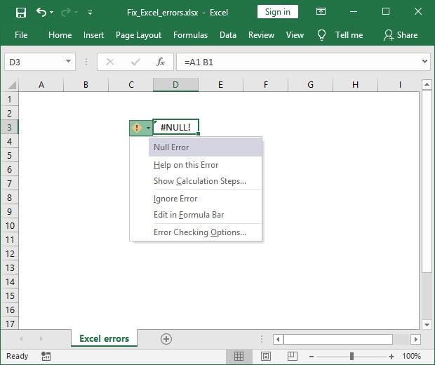
As you can see, the green triangle is visible in my cell because Excel has displayed a #NULL! error. A yellow diamond shape has appeared, which can be pressed to display Excel’s error menu.
So, what exactly is this menu used for?
- The gray row tells us which error has been triggered.
- The “Help on this Error” link will open Excel’s help panel, where you can find hints on how to fix your error.
- The “Show Calculation Steps…” link will prompt the Evaluate Formula panel, where you can check every step of your formula and see which one is triggering the error.
- The “Ignore Error” link does precisely that – it removes the green triangle from your cell and ignores the error.
- The “Edit in Formula Bar” link takes you to the formula bar to modify your formula.
- “Error Checking Options…” link opens the Error settings. Here, you can tweak and customize Excel’s settings related to how errors are displayed and what type of errors to look for and reset the ignored errors from your workbook.
Excel displays nine types of errors (eight if you are not using Office 365 or Office 2021), and you should understand what triggers them and how to fix your broken formula.
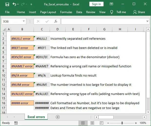
Fixing errors
Fixing your Excel errors is a multi-step process. Remember that even though a cell shows an error, it doesn’t mean that it’s the cell causing it. Often errors cascade from one cell to another or even from different sheets or workbooks. If you fix the underlying error, all the other formulas will be fixed as well. Here is the five steps process I use for fixing my Excel errors:
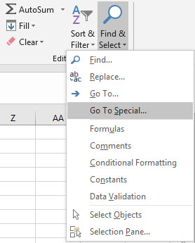
1. Finding the errors. You can use Go to Special > Formula by pressing Ctrl + G and then selecting Special. Alternatively, you can go to the Home tab, Editing, and Find & Select as shown below.
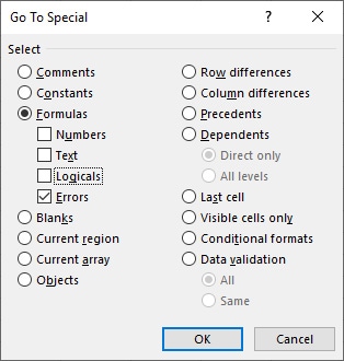
2. Select all cells with errors using the Go To Special menu. This way, we can see all cells which return error messages.
3. Trace the error back to its source. The Formula Auditing menu provides excellent features to trace back errors to the source or check which cells are propagating your errors.
4. Figure out what’s causing the error. If you have a complex formula, it can be a good idea to break it down into smaller parts. You can also use the Evaluate Formula option and see which step generates the error.

5. Fix the source of errors. When you find the cell causing the error and fix the formula, all your other dependent errors will get fixed.
#REF! error in Excel
I get asked a lot, “what does #REF! mean in Excel?” The #REF! error is very common and shows up when a formula refers to a cell that is not valid. Usually, the cell has been deleted, or other cells have been pasted over (using cut and paste). If you see #REF errors appearing after you delete a row or a column, it is wise to click Undo (or use the shortcut Ctrl + Z), evaluate your formula, and decide whether you should replace that cell or remove it.
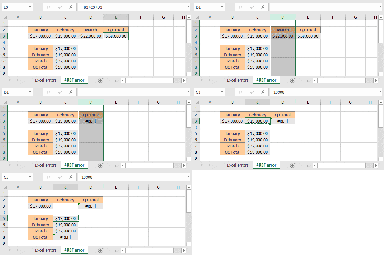
The easiest way to prevent #REF! errors is to check for dependent cells. You can easily see all the cells that link to the cell you want to delete by using the Trace Dependents option in the Formula Auditing section of the Formula Tab. This way, you will know which formulas will be affected if you delete a specific cell from your worksheet.

#REF! error while using VLOOKUP or INDEX
VLOOKUP and INDEX functions can also generate #REF! errors whenever you use incorrect range references. For example, if you specify a value for the col_index_num parameter, which is higher than the total number of columns in your table, VLOOKUP and INDEX will return a #REF! error message.
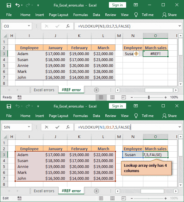
If you ever encounter #REF! errors within your lookup formulas, the first thing you should do is check your parameters and correct them. Use caution when you delete columns from a range that serve as the table_array argument because they will break your VLOOKUP formulas. A safe approach would be to switch from a hardcoded value to a relative approach using the MATCH function.
#REF! error while using INDIRECT
For those of you who use INDIRECT to create dynamic links, please note that referencing a closed workbook in an INDIRECT formula will result in a #REF! error. In this case, opening the linked workbook will remove the error, and your formula should work correctly. Please note that closing the linked workbook will trigger the #REF! error again.
#REF! error while linking to another Excel file
Whenever you work with files saved on a server or shared location, there is a high chance you will run into this error. If your link turns into something like [Test_link.xlsx]#REF'!$B$2 after opening a linked file, then you should know there aren’t many options to restore your formulas. Your best bet is to close your file without saving it. When you reopen it, the error will not be there.
If you have saved your file then all your links will be transformed into #REF and you will not be able to revert them. In this case, restore a previous version of your file or use a locally saved backup.
Now, let me explain what is actually causing this so you can avoid it. For some reason, when you are using a shared location to save your files, Excel is having a hard time recognizing other workbooks that are linked to your current file. So, if you are opening a workbook directly from Windows Explorer (i.e. like you normally open files in Windows) and that file is linked from the current opened Excel workbook, it will generate #REF errors.
To avoid this, once you have linked to a file in your workbook, make sure you only open it from the Data tab, using the Edit Links option.
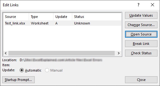
This tip alone will save you a lot of time, because if you mess up your formulas and don’t have a backup, then you will have to manually recreate them (which can be a pain).
#VALUE! error in Excel
This is probably the most common error code. Whenever you encounter a #VALUE! error in Excel it means that something is wrong with the cells you are referencing.
The most frequent solution is to check for different data types in your formula. For example, trying to add a number (i.e. 27) with a text cell (i.e. John) will result in a #VALUE! error message. Now, I know you are not adding numbers with text, but there are scenarios when you may be doing it without even knowing it. For example, if you work with large data sets or download a database from your CRM, they may contain data that looks like numbers but it is in fact stored as text.
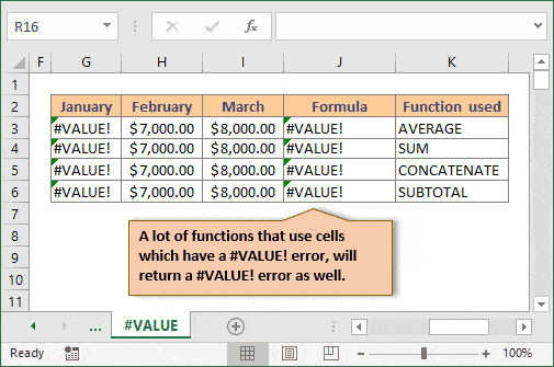
Also, referencing cells that have #VALUE! errors will cause most of the functions to return a #VALUE! error as well. Below you can see how AVERAGE, SUM, CONCATENATE, and SUBTOTAL return errors just because they are using the input from column G which returns a #VALUE! error. So, if you can’t figure out why your formulas are returning a #VALUE! error, make sure you also check your input.
#VALUE! error while subtracting
If you are using the Windows version of Excel you might get the #VALUE! error when writing basic subtraction formulas. If a simple formula like =B3-C3 returns a #VALUE! error, then you will have to check Windows Region and language settings. To learn more please refer to this official article from Microsoft.
#VALUE! error while using COUNTIF or COUNTIFS
There are three main reasons why COUNTIF or COUNTIFS will return a #VALUE! error. The first one, and most often, is caused by formulas that link to cells in closed workbooks. However, COUNTIF and COUNTIFS functions will not always return #VALUE! error when linking to closed workbooks. From my experience, this happens most often when you are working on a remote environment like SharePoint or an external server. This is a known issue with other Excel functions like COUNTBLANK, SUMIF, or SUMIFS.
How to fix this #VALUE! error? Simply open the linked workbook from your formula, and then press F9 to refresh the formula.
The second reason why COUNTIF will throw in the #VALUE! error is related to your search string. Keep in mind that Excel cannot use a string longer than 255 characters as your search criteria in COUNTIF function. This means that you will have to shorten the string used in your COUNTIF or COUNTIFS formula in order for the functions to work correctly.
The third reason why COUNTIFS will return a #VALUE! error is inconsistent range referencing in your formula. For COUNTIFS (and also SUMIFS), you need to make sure that a similar range of cells is supplied in all the Range/Criteria pairs. For example, a formula like =COUNTIFS(B1:B10, ">="&A1, C1:C12, "<="&A2) because either the first range should be extended to B1:B12 or the second one should be shortened to C1:C10. Otherwise, your formula will keep returning the #VALUE! error message.
#VALUE! error while using SUMPRODUCT
If you are working as an analyst and you are not using SUMPRODUCT then you are missing out. SUMPRODUCT is one of the most powerful and useful functions and I cannot stress this enough. It is versatile and can be easily used to create subtotals based on multiple criteria, it can replace SUMIFS and COUNTIFS, and it can even perform lookups.
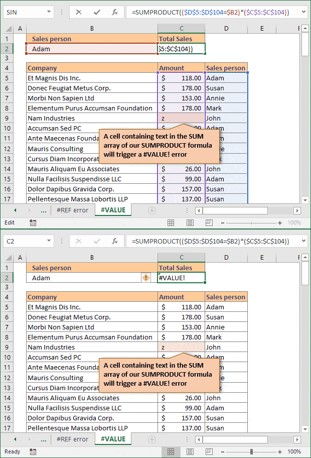
However, if your SUMPRODUCT formulas are returning a #VALUE! error, then it means that somewhere in the arrays you have at least one cell containing text. This can be a table header, a comment column, or even a single letter typed by mistake in your array. I am sure you accidentally typed in a Z when trying to use the Undo shortcut Ctrl + Z.
#VALUE! error while using VLOOKUP
If you work with VLOOKUP and your formula returns a #VALUE! error then there are two possible causes.
- The lookup_value argument is more than 255 characters. The quick solution is to shorten the lookup value. If you can’t use this approach, then use a combination of INDEX and MATCH functions as a workaround.
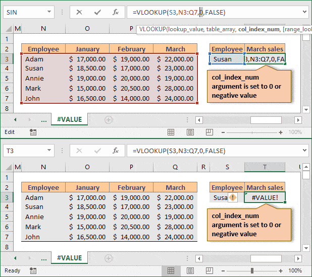
- The col_index_num argument contains text or is less than or equal to 0. Make sure you didn’t insert a negative value or zero by mistake. It’s easy to type 0 instead of 10 or insert additional letters. Double-check your formula and correct any input mistakes.
#DIV/0 error in Excel
What does #div/0 mean in Excel? Well, since dividing by zero will result in no mathematical result that Excel can display, it will trigger a #DIV/0 error message. Whenever you see this message, it means that you are either dividing by a cell that is blank (and treated as zero) or part of your formula that is treated as the divisor equals zero. In order to fix it evaluate your formula and check which part is triggering the error.
#N/A error in Excel
A lot of people are asking me “why is my formula not working?”, “what does #N/A mean in Excel?”, “how to hide #n/a in Excel?” The #N/A error is Excel’s way of telling you that your formula can’t find what you are looking for. This is most common with VLOOKUP, HLOOKUP, LOOKUP, and MATCH functions.
If you are looking at how to hide error messages returned by Excel, please read along. The final part of the article explains the best way to approach error messages in Excel.
#N/A error while using VLOOKUP, HLOOKUP, LOOKUP or MATCH
If you are using exact match for your lookup functions, then the #N/A error means that no matching result has been found. In order to fix the error, check your data series manually. If the value you are looking for exists, then it means that there may be additional spaces before or after your data.
For Excel, an exact match means that the strings need to be identical. So, if you are looking for “Jane” but your data series contains ” Jane” (two spaces before the text), then Excel will return #N/A because the two strings are considered different.
Most of the time all you need to do to prevent #N/A errors is to make sure that the lookup value is correct and that your lookup tables do not have data with ending spaces. In some cases, it can even be useful to trap the error using IFERROR and display a more friendly message (or just hide the error). The final section of this article describes the use of IFNA, IFERROR, and ISERROR to hide errors or display custom messages.
#NAME? error in Excel
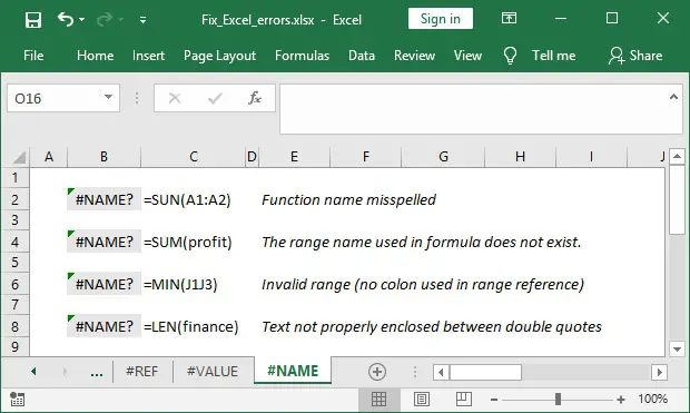
The #NAME? error indicates that Excel is not able to recognize part of your formula. It may be that you have misspelled a function name, you are referencing a named range that doesn’t exist, or simply entered a wrong cell reference.
Function name misspelled
Misspelling a function name will make Excel unable to recognize your formula and display a #NAME? error. For example, =SUN(A1:A2) is not a valid formula because the name of the function is not spelled correctly.
The range name used in the formula does not exist
Another common mistake is using a range name that isn’t available or misspelling a range name. Most often this happens if you accidentally remove one of your named ranges and Excel is not able to recognize them anymore. Make sure that you double-check your ranges before you delete them.
Invalid range
If you are manually writing the range in your formula (as opposed to selecting it with your mouse or keyboard), you may run into a #NAME? if you forget to use a colon when defining your range. In the example above the MIN function is using an invalid range. The correct range reference is J1:J3, so Excel will return an error.
Text not properly enclosed between double quotes
When you work with functions that handle text you have to make sure that you are enclosing your input between double-quotes. Otherwise, Excel will not be able to recognize it as a text. In the example shown above, the LEN function is not able to return the correct result because the input should be "finance" and not finance.
##### error in Excel
The most probable reason why Excel is displaying ##### instead of your input or result is that the column isn’t wide enough to show all of the cell contents. Increase the width of the column and the error should go away. Also, try reducing the number of decimals, decreasing the font size, and increasing the zoom. This will allow for more content to be displayed.
Alternatively, the ##### error can be caused by formulas that subtract dates or times. In Excel, negative values for dates and times are always shown as #####. To avoid this, try using date functions as much as possible when working with dates. For example, instead of just subtracting two dates try using a function like DATEDIF.
#NULL! error in Excel
Well, the #NULL! error isn’t something you will see very often. It basically means that you have incorrectly separated cell references in your formulas. For example, the formula =SUM(A1 A10) will return a #NULL! error because the range lacks the colon “:” or comma “,” between the two cell references. All you need to do is adjust the range to A1:A10 or separate the two cells by a comma and the error will go away.
#NUM! error in Excel
What does #NUM! mean in Excel? Well, the #NUM! error is displayed when a number is too large or too small, or when a calculation isn’t possible. For example, it’s impossible to display 10^3000 because it is too large. Alternatively, if you are trying to calculate the square root of a negative number Excel will return a #NUM! error because this is impossible from a mathematical point of view.
#SPILL error in Excel
#SPILL error only applies to Office 365 and Excel Online. Basically, Excel is telling you that the spill range for a spilled array formula isn’t blank. You can read more about this error on Microsoft’s website.
How to hide error messages in Excel using IFERROR, ISERROR, or ISNA
Sometimes you may get errors as part of the normal data analysis. An #N/A error in a VLOOKUP formula isn’t necessarily bad. It just tells you that the value you are looking for couldn’t be found in the table array. However, that doesn’t mean #N/A errors are pretty and that is why it makes sense to replace them with a custom message like “value not found” or hide them altogether.
One word of caution though: verify that your formulas are correct before you trap and hide the errors. There is nothing worse than hiding a formula result because it generates an error created by a poor formula/data. For example, a VLOOKUP might return an #N/A error because there are beginning or ending spaces in your lookup value or table array. However, the value exists, and hiding the error rather than fixing will return a wrong result.
Below I will show you 3 examples of how you can customize your error messages for a VLOOKUP formula. These can be applied to any formula you desire.
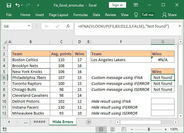
Your first option is to use IFNA function. This is perfect for displaying a custom message like “Not found” for your VLOOKUP formulas because the IFNA function only replaces your #N/A errors. In cell G6, I have used the formula =IFNA(VLOOKUP(F3, B3:D12, 3, FALSE),"Not found"). If the lookup value cannot be found (in our example Los Angeles Lakers is not included in the table array), then the formula will return an #N/A error. The IFNA formula result will be TRUE and the custom message will be shown. Alternatively, you can remove the custom message and just insert “” and Excel will display a blank cell (like cell G10).
The second option is to use IFERROR function. In cell G7 we have the formula =IFERROR(VLOOKUP(F3, B3:D12, 3, FALSE), "Not found") which will trap any error generated by our VLOOKUP, not just #N/A. For example, if you have a #VALUE! error while using VLOOKUP the message displayed will be the same as for the #N/A error. However, the #VALUE! error should be fixed and not hidden as a “Not found” message.
The third option is to use the IF function with ISERROR. This will achieve the same result as IFERROR but will also work in older versions of Excel. In our example, cell G8 contains the formula =IF(ISERROR(VLOOKUP(F3, B3:D12, 3, FALSE)), "Not found", VLOOKUP(F3, B3:D12, 3, FALSE)). This works pretty much like any other IF formula. If the condition is TRUE (the VLOOKUP formula returns an error) then display “Not found”, otherwise display the result of the VLOOKUP formula.
I hope that after reading this article you are much better equipped to identify the cause of your Excel errors. If you want, you can also download the file I used in this article.
Where do you struggle with Excel formula errors? Drop me a message in the comments section below.
