How to use INDEX and MATCH functions in Excel

July 11, 2024July 11, 2024

I know a lot of you may think that VLOOKUP is all you need to perform a lookup. However, understanding the principles of how to use INDEX and MATCH functions in Excel will yield more benefits than you think. I am not saying you should replace VLOOKUP completely, but rather know its limitations and when to switch to an INDEX-MATCH approach.

Whenever I ask people why they do not use INDEX MATCH instead of VLOOKUP, they tell me that it requires two functions, one nested inside another, and that this is confusing. I am here to tell you that you will find it a lot easier to write your own INDEX-MATCH formulas once you read this tutorial. After all, if you want to take your Excel skills to a new level, you have to learn how to combine multiple functions and write complex formulas.

How to use the INDEX function in Excel

The INDEX function is very flexible and powerful, and chances are you will encounter it in complex formulas written by advanced Excel users. So, what does INDEX do? Simply put, INDEX retrieves the value from a given table.

Let’s take a quick look at the syntax of INDEX and its arguments:
=INDEX (array, row_num, [col_num], [area_num])

array – A range of cells or an array constant.
row_num – The row in the array from which to return a value.
col_num – [optional] The column in array from which to return a value.
area_num – [optional] The range in reference that should be used.

The following example shows the basic use of INDEX function.

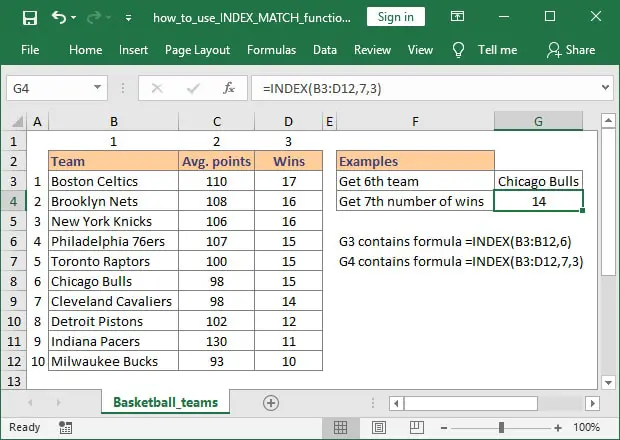
Assume we have a table with 10 basketball teams and we want to get the name of the 6th team from our list. A quick INDEX formula can retrieve this for us:
=INDEX(B3:B12, 6)

As you can see, out of the four arguments we only had to use two: array and row_num. Since we only had one column of data there was no need to use the col_num argument.

In cell G4 we have another INDEX formula to retrieve the number of wins for the 7th team. The formula is again very simple:
=INDEX(B3:D12, 7, 3)

We are telling Excel to look in our array (B3:D12) and select the cell from the intersection of row 7 and column 3, which is D9. Remember that INDEX is only looking at your defined array and not the entire sheet.

You may think “What is so great about this? Can’t I just select that cell in the formula manually, since I already know what value I need?” Well, this is when the MATCH function comes into play and makes things interesting.

How to use MATCH function in Excel

MATCH is used to locate the position of a lookup value in a row, column, or table. It supports both exact and approximate matching, as well as wildcards (* ?) for partial matches.

The MATCH function has 3 arguments:
=MATCH(lookup_value, lookup_array, [match_type])

lookup_value – The value that you want to match in lookup_array;
lookup_array – A range of cells where to search for the lookup_value;
match_type – [optional] The type of matching used, specified as -1, 0, or 1.

The lookup_value argument can be a value (number, text, or logical value) or a cell reference to a number, text, or logical value. One thing to remember is that MATCH returns the matched value position within lookup_array, not the value itself.

MATCH has several matching modes, and when used with other functions (like INDEX), it creates a more flexible lookup alternative to VLOOKUP or HLOOKUP.

Match types

There are three values you can supply for match_type, based on what you need to match.

• If you use match_type 1, then MATCH will find the largest value lower than or equal to the lookup_value. The values in your lookup_array argument must be placed in ascending order.
• If you use match_type 0, then MATCH will find the first value that is exactly equal to lookup_value.
• If you use match_type -1, then MATCH will find the smallest value greater than or equal to lookup_value. The values in your lookup_array argument must be placed in descending order.

There are a few things you should remember when working with MATCH:

• All match_types (-1, 0, 1) will return an exact match if one exists.
• If you omit match_type, Excel uses the default value of 1.
• If MATCH is unsuccessful in finding a match, or if your data is not sorted properly (ascending or descending based on match_type), Excel will return the #N/A error value.

Now let’s return to our previous basketball example.

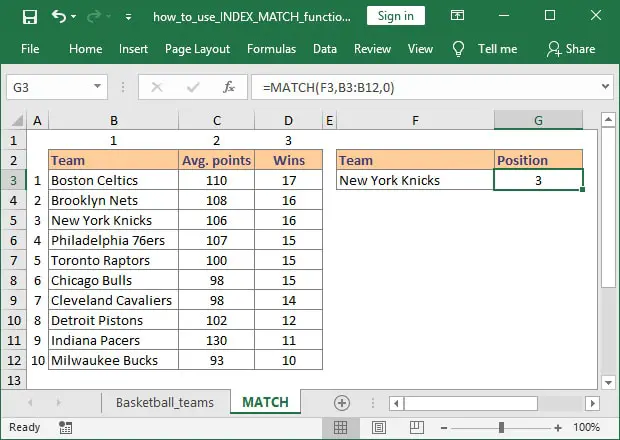
Using the formula =MATCH(F3, B3:B12, 0) we can return the position of the lookup_value (in this case, the New York Knicks) in our range (B3:B12).

Using INDEX and MATCH together

The final step is to combine those two functions into one strong lookup formula. You can achieve this fairly easy, once you understand how it works. We will use the INDEX function and define the row_num and col_num arguments using MATCH.

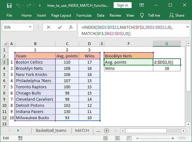
You can see below the formula I used to retrieve Average points per game:
=INDEX($B$3:$D$12, MATCH($F$2, $B$3:$B$12, 0), MATCH($F3, $B$2:$D$2, 0))

You start with the array the argument of INDEX which defines the area where your formula will lookup your value, in our case $B$3:$D$12.

Then, you add the first MATCH, which is used to identify the row where our lookup_value (cell F2) is located.

The final part of our formula uses another MATCH to determine which column to use in the INDEX function. In this example, I needed “Avg. points” and for that, I compared cell F3 with the table heading $B$2:$D$2.

All examples from this article work in Excel for Microsoft 365 or Excel 2019, 2016, 2013, 2010, and 2007.

Why INDEX MATCH is better than VLOOKUP

A formula based on INDEX and MATCH can achieve everything VLOOKUP can do and more. It’s simply faster and more flexible and has a lot of benefits:

• It can look both vertically and horizontally
• It can look left or right (VLOOKUP only looks right)
• Adding more columns to your table won’t break the formula (like it sometimes happens with VLOOKUP)
• When you have a large set of data, it can be faster than VLOOKUP
• It can work with data sorted in descending order (VLOOKUP can only be used with data sorted in ascending order)

I am a big fan of INDEX and MATCH formulas, but I also use VLOOKUP whenever convenient. Sometimes keeping things simple is the best approach, and there isn’t a good reason to stop using VLOOKUP just because you learn how to use INDEX and MATCH. Below are a few of the benefits of using VLOOKUP:

• it’s friendly with beginners but still provides a great way of performing lookups
• it’s easier to configure and requires only one function
• it’s easier for others to understand your formulas

Please let me know if you have any questions by posting a comment.