How to use COUNTIF function in Excel
In this article, I will focus on how to use COUNTIF function in Excel. The purpose of COUNTIF is to count cells that meet a single criterion. If you need more criteria in your formula, then the COUNTIFS function is a much better option.
How to use the COUNTIF function
COUNTIF applies criteria to a given range, counts the number of occurrences matching the criteria, and returns the number of matches. The syntax is:=COUNTIF(range, criteria)
The function uses only two arguments:
range – The range of cells you want to count. The range can contain numbers, arrays, a named range, or references that contain numbers. Blank values are ignored.
criteria – The criteria used for counting. This can be a number, expression, cell reference, or text string.
COUNTIF is not case-sensitive and will treat all text the same way. This means that using “Orange”, “orange” and “OrAnGe” will return the same result. However, you can combine COUNTIF with the EXACT function if you are looking to apply case-sensitive criteria.
Examples of COUNTIF formulas:=COUNTIF(A1:A12, 30) – counts cells equal to 30=COUNTIF(A1:A12, "<>30") – count all cells different from 30=COUNTIF(A1:A12, "orange") – counts cells equal to “orange”=COUNTIF(A1:A12, ">="&C1) – count all cells higher than or equal to the value in cell C1
Note: Since the operators need to be entered as text between double quotes (“>=”, “>”, “<=”, “<>”), we have to use the ampersand symbol (&) to concatenate the operator with the criteria cell. If you skip this step, Excel will not be able to understand your formula and will display an error message.
The following image shows you the basic use of COUNTIF. In the table I have entered the last 12 games played in 2018 by the Golden State Warriors (NBA team), the points scored in each game, and the result. The formula =COUNTIF(D5:D16, "W") counts how many wins they had.
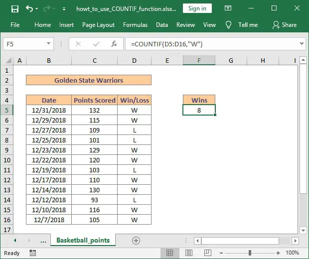
Excel COUNTIF function examples
As you have just seen, using the COUNTIF function in Excel is very easy. However, the flexibility of the function allows for many criteria, including wildcard characters for partial matching, named ranges, other cell references, and even the use of other Excel functions. COUNTIF is truly a powerful function that can be used in a wide selection of real-life situations.
COUNTIF greater than, less than, or equal to a value
If you need to count cells with values greater than, less than, or equal to a specific number, all you need to do is add the corresponding operator to the criteria.
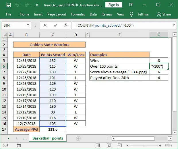
Looking back at our Golden State Warriors example, we can count the number of games where the team scored more than 100 points. The formula to achieve this is very simple and uses the ">" operator:=COUNTIF(points_scored, ">100")
In this example, I have used the named range points_scored (cells C5:C16). If you are using manually inserted numbers (instead of a cell reference) you will need to enclose them in quotes "" along with the operator.
Below you can see examples of formulas using the numeric operators available with COUNTIF function:=COUNTIF(C5:C16, ">100") – Counts all greater ">" than 100;=COUNTIF(C5:C16, "<100") – Counts all cells lower "<" than 100;=COUNTIF(C5:C16, "<>100") – Counts all cells not equal "<>" to 100;=COUNTIF(C5:C16, "=100") – Counts all cells equal "=" to 100;=COUNTIF(C5:C16, "<=100") – Counts all cells lower than or equal "<=" to 100;=COUNTIF(C5:C16, ">=100") – Counts all cells higher than or equal ">=" to 100.
COUNTIF using another function in the criteria
Learning the basics is important, but understanding how to use COUNTIF function in Excel along with other functions will yield great benefits. Below I have prepared two examples of how to use COUNTIF with AVERAGE and DATE functions.
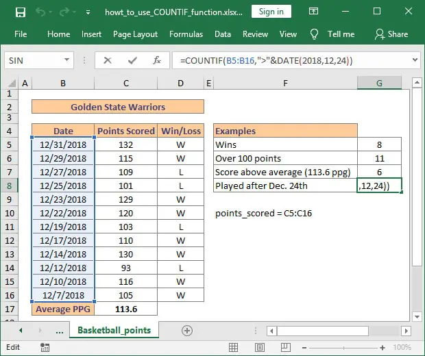
As you can see, the Average Points per Game for the Golden State Warriors is 113.6 (cell C17). Using the AVERAGE function we can count in how many games they have scored more points than their average PPG. The formula is very simple:=COUNTIF(points_scored, ">"&AVERAGE(points_scored))
Taking the example a bit further, I have used COUNTIF and DATE functions to return the number of games played after December 24, 2018. The formula used to achieve this is straightforward:=COUNTIF(B5:B16, ">"&DATE(2018,12,24))
Please note the use of the ampersand symbol (&) to concatenate the operator with the criteria.
COUNTIF formula with wildcard characters for partial matches
Often times your Excel data will include variations of the words you want to count and using an exact match formula will not return the correct result. This is why learning to use wildcards with COUNTIF is so important. The use of wildcards allows you to count all the cells containing a certain string (word, phrase, or letters).

Now let’s look at an example. Suppose you have a list of sales, aggregated from several sources. This means that different people may use different input when they record data. In our case, we have several variations for the name Sara Parker. If we want to count the number of sales completed by Sara, we will have a hard time using an exact match formula. The formula to count all cells which contain the string “Parker” is shown below:=COUNTIF(B3:B10, "*Parker*")
The use of the asterisk "*" wildcard before and after the search term means that we want to count all cells which contain “Parker”, regardless of the position of this string (beginning with, ending in, or in the middle of the text). If you need to match a single character, use the question mark "?" wildcard instead.
Count cells beginning or ending with certain characters
The second example I have prepared demonstrates the use of wildcards to count all cells which have text ending with our search term.
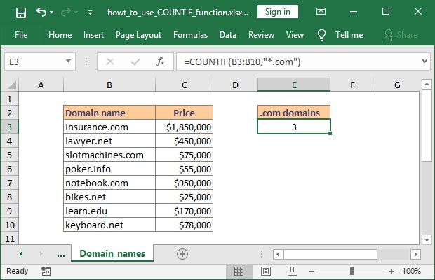
Above is a list of domain names and their estimated sale price. Counting all .COM domain names from the list can be achieved really fast using the following formula:=COUNTIF(B3:B10, "*.com")
If you need to count cells that start with a certain string just move the "*" at the end of the criteria and you are good to go. For example, using “Dan*” will count all cells which contain the string “Dan” at the beginning of the text. This includes “Dan” but also variations such as “Daniel” or “Danny”.
Excel COUNTIF for blank and non-blank cells
There may be times when you need to count the number of cells which are blank or the number of cells that hold data, regardless of their content.
COUNTIF if cell is not blank
In one of my projects, I had to use license keys for a lot of different products. Since those license keys were delivered to me as .txt files, the easiest way for me to keep track of them was to import them into an Excel file. After each sale, I removed the key from the list of available licenses. In order to keep track of unsold inventory, I created a formula based on COUNTIF function, which counted all cells which had text (any characters). For this I used the following formula:=COUNTIF(range, "*")
There is however a catch with this formula. It works only for cells containing text because it ignores entries such as numbers or dates. If you are looking to count cells that contain any type of input you can use:=COUNTIF(range, "<>"&"")
COUNTIF cell is blank
Counting blank cells is just as easy. All you need to do is use the formula =COUNTIF(range, ""). The formula correctly handles numbers, dates, and text values.
As an alternative, Excel has a built-in dedicated function to count blank cells, called COUNTBLANK. The syntax is very simple. with only one argument – the range where you want to apply it. The syntax is:=COUNTBLANK(range)
What to do next?
I hope that after reading this article you have a much better understanding of how to use COUNTIF function in Excel.
Please let me know if you have additional questions by posting a comment.
