How to find duplicates in Excel using Conditional Formatting
While working with large Excel worksheets or consolidating several files, you may need to check for duplicates. Depending on the task at hand you could be faced with a wide variety of situations. This article describes the most common examples you may encounter and how to find duplicates in Excel.
If you are looking for a different approach, I have also posted an article on How to find duplicates in two excel sheets.
How to find duplicates in Excel
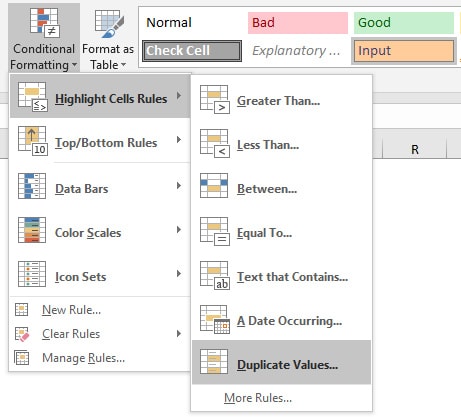
Conditional Formatting is a very versatile tool. It has pre-defined conditions but you can also use formulas for more complex tasks. You can find the Conditional Formatting in the Home tab, under the Styles section. If you select Highlight Cells Rules/Duplicate Values, Excel will highlight all cells which are found at least twice.
Please keep in mind that this approach works best when you have a unique identifier to distinguish between different database entries.
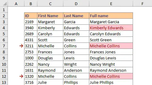
Our example file contains a database with users. When they registered, they provided their First name and Family name and the system generated an ID. Now, let’s assume that we used several sources to create this table in Excel and some of the users appeared more than once. Using the Duplicate Values option on column E, we can highlight the users with the same name.
However, looking closer we can see that there are some users with the same name but different IDs. This means that using the pre-defined “Duplicate Values” Conditional Formatting is not good enough in this case. Simply deleting the highlighted values based on the name criteria would result in losing data.
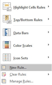
A better approach is to check the full entry (ID + Full name) by creating a Conditional Formatting rule using a formula. To do so, simply select the area where you want to apply the Conditional Formatting rule. In my case this is range $B$3:$B$202. Then, navigate to the “Conditional Formatting” tab and click on “New Rule”.
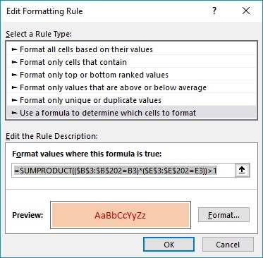
Choose “Use a formula to determine which cells to format” as the Rule Type and insert the formula you want to use. Don’t forget to change the formatting of the cells in the Format tab. My rule contains the following formula:=SUMPRODUCT(($B$3:$B$202=B3)*($E$3:$E$202=E3))>1
How the SUMPRODUCT formula works
In case you are not familiar with the SUMPRODUCT formula, I strongly recommend taking the time to learn it. I assure you it has a lot more uses than looking for duplicates in Excel.
SUMPRODUCT returns the sum of the products of ranges or arrays. While this may not sound like much, keep in mind that SUMPRODUCT is a versatile function and can be used in a wide variety of situations. This incredible function can be used to count or sum items based on criteria (like COUNTIFS or SUMIFS) but provides a lot more flexibility.
Syntax and arguments of SUMPRODUCT:=SUMPRODUCT (array1, [array2], [array3], ...)
array1 – The first array or range to multiply, then add.array2 – [optional] The second array or range to multiply, then add.array3 – [optional] The third array or range to multiply, then add.
While SUMPRODUCT function uses arrays, it does not require the standard array syntax (Ctrl + Shift + Enter) to enter. SUMPRODUCT will behave exactly like the SUM function when only one array is supplied. Keep in mind that SUMPRODUCT supports up to 30 arrays.
SUMPRODUCT assigns a value of 1 when the criteria are met, or a value of 0 when the criteria are not met. Then, it sums all the values and returns the total. Using “*” sign in the formula makes the two conditions cumulative.
Understanding the Conditional Formatting formula
The easiest way to understand how to find duplicates in Excel with this conditional formatting formula is to split it into three parts.
Part one and two checks to see if cells from arrays ($B$3:$B$202) and ($E$3:$E$202) match the values from cells B3 and E3 respectively. If they are both true, then it will return a value of 1.
Part three checks if the sum resulted from SUMPRODUCT is greater than 1. The conditional formatting formula will then move to the next set of cells, B4 and E4, and perform the same checks, then continue all the way down to row 202.
A simple way of looking at this formula would be:
a) SUMPRODUCT will check if ID from cell B3 is found in the array $B$3:$B$202 and generates an array with only 1s and 0s: {1, 0, 0, 1, ... , 0, 1}.
b) SUMPRODUCT will check if the Full name from cell E3 is found in the array $E$3:$E$202 and generates the second array: {1, 0, 0, 0, ... , 1, 0}.
c) SUMPRODUCT will multiply these two arrays and return the sum: {1*1 + 0*0 + 0*0 + 1*0 + ... + 0*1 + 1*0}.
d) The formula will check if the result returned by SUMPRODUCT is greater than 1 (remember our “>1” condition).
If the value is greater than 1, this means that the combination of ID + Full name is not unique in our table.
Note: Keep in mind that all the arrays in the SUMPRODUCT formula must be the same size. Otherwise, SUMPRODUCT will generate a #VALUE! error.
The result of our two Conditional Formatting rules
When you apply the new rule, it will highlight all the cells that match the result of our formula. In this example, I mentioned that there are some entries that have the same name, but the ID is different. This can be the case when two people with the same name register on a website or if two employees have the same name. They will have different IDs but the same name.
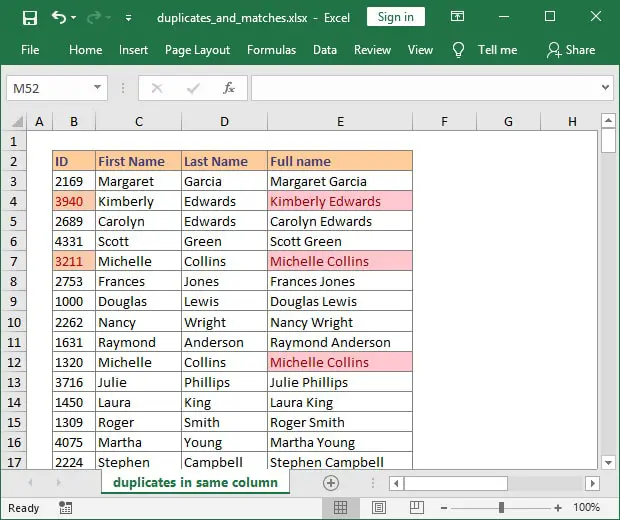
SUMPRODUCT formula, while cells from column E are highlighted using the built-in Excel conditional formatting. In the case of “Michelle Collins” the file contains 3 entries. Two of them are duplicates (rows 7 and 27), but there is another entry (row 12) that is unique. Highlighting the cells based solely on the name would result in a false highlight in this case.
This formula can provide an easy way to find duplicate rows as well. Just add more conditions to the SUMPRODUCT formula and it will reveal all your duplicates.
If you have additional questions or need help with your project, please let me know by posting a comment.

Hi there,
First off, this was very helpful! I used this formula for three different arrays with a column in between them (D,F,G). Column E is a description that can often get keyed in differently by different users so it was not included. The formula works, finds duplicates, and highlights them in column D. The issue I’m having is that all sorts of values in column F are being highlighted as well. No rhyme or reason to which ones are highlighted but it is a lot. I’m curious how to fix this. Any suggestions would be much appreciated!
Hi Lauren,
It’s hard to tell without seeing the file, but I would start by checking the Conditional formatting for one of the cells wrongly highlighted in column F. Look for the cell references and make sure they’re the same for all arrays. If one array is using relative reference and the others are using absolute reference, it may break your formula and mess with the Conditional formatting rules along the way.
Also, I usually suggest applying the Conditional formatting rule for just one column to avoid excessive highlighting and validation checks which may slow down the file. Is highlighting column F is really necessary?
Last, but not least, keep in mind that copying a cell and pasting it in a different place will also copy the Conditional formatting rules. Have you copied any cells from one column to the other?
Let me know if any of these help.
Hi Radu,
The cell references were the same for all arrays. I don’t actually need multiple columns to be highlighted so I just changed the formatting rule to apply to just column D. I think I was worried excluding the other columns would mess with whether the formula pulled values from them to verify duplicates, so I’m happy to see that the formula works just fine with one column!
Thanks so much for your prompt response and help. I’m happy to add this functionality to this file!
Hi Lauren,
I’m glad I could help.