How to use SUMIF function in Excel
SUMIF is considered one of the important Excel functions to learn. This tutorial explains how to use the SUMIF function in Excel, and it’s intended to be a comprehensive guide with many real-life SUMIF formula examples.
SUMIF adds more functionalities to the basic SUM formula by introducing selection criteria. The SUMIF function returns the sum of all the cells from a range when the supplied criteria is met. This means that you can take a range and only add up certain cells while completely ignoring the rest.
SUMIF syntax in Excel
The SUMIF syntax is really simple and only uses three arguments:
=SUMIF(range, criteria, [sum_range])where
- range (required) – The range to compare against the criteria.
- criteria (required) – The criteria to use on the range.
- sum_range (optional) – The range containing the values to be summed. If omitted, then the values from range are summed.
The SUMIF function supports logical operators (>, <, <>, =) and wildcards (*, ?) for partial matching.
If you want to apply multiple criteria, I recommend using the SUMIFS function.
How to write a basic SUMIF formula in Excel
Now let’s look at a few SUMIF examples. Let’s calculate the total sales of pizza.
To write the SUMIF formula, follow these steps:
- Type =SUMIF( to activate the function.
- Select the range to compare against the criteria. In this example, it is C3:C12.
- Insert the criteria to be used in the SUMIF formula. I have used “Pizza” since we only want to sum the cells with pizza sales.
- Select the range containing the values to be summed. In my example, this is the range D3:D12 which contains all the sales from our example.
- Close the parenthesis ) and press to finish the formula.
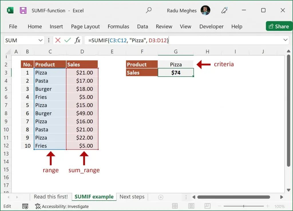
The formula I ended up with is:
=SUMIF(C3:C12, "Pizza", D3:D12)Note: If you use text criteria, you need to wrap them inside double quotation marks. Also, logical operators need to be enclosed in double quotation marks (e.g. “<15”).
Alternatively, the same result can be achieved by including the criteria using a cell reference:
=SUMIF(C3:C12, G2, D3:D12)These simple formulas use the SUMIF function to return only the sum of pizza sales while ignoring the rest of the data.
Sum if equal to
A sum if equal to the formula is the easiest and works with numbers and text. The formula doesn’t require the equal sign, as this is how the SUMIF Excel function is built.
Let’s say we want to calculate the total orders placed by customers that dined in Table 1. We can write a simple SUMIF formula that looks like this:
=SUMIF(E3:E12, 1, D3:D12)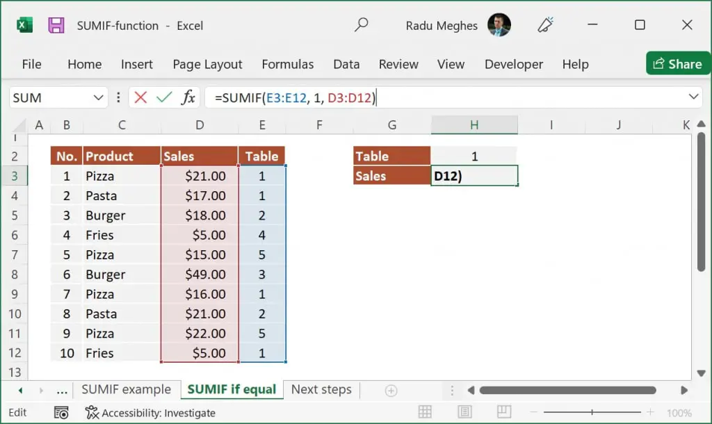
If you prefer, you can also write this formula as:
=SUMIF(E3:E12, "=1", D3:D12)The results are the same in both cases.
You can also replace the hardcoded criteria with a cell reference to make your formulas dynamic. In this case, the SUMIF formulas would look like this:
=SUMIF(E3:E12, H2, D3:D12)where:
- the criteria range E3:E12 contains the list of tables
- the range D3:D12 contains the corresponding cells with the sales amounts
- cell H2 contains the table number
The initial example from this article showed you how to sum cells based on text input. The only difference is that you need to enclose the string between double quotation marks like this:
=SUMIF(C3:C12, "Pizza", D3:D12)Note: You don’t need the double quotation marks when using cell references as the criteria argument.
Sum if not equal to
When writing a SUMIF not equal to a criteria formula, you need to use the “not equal to” logical operator (“<>”). If you hardcode the value for the criteria argument, wrap it around double quotation marks (e.g., “<>Pizza” or “<>3”).
Now let’s look at a simple formula that doesn’t use a cell reference for the criteria argument. We will calculate the total sales for orders that don’t include Pizza. The SUMIF formula is:
=SUMIF(C3:C12, "<>Pizza", D3:D12)To use cell references, you need to concatenate the criterion with the “not equal to” logical operator like this:
=SUMIF(C3:C12, "<>"&H2, D3:D12)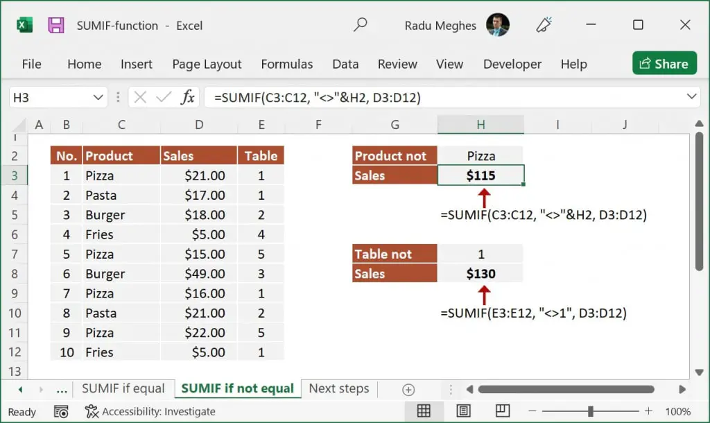
Note: only the logical operator is enclosed between double quotation marks. The ampersand symbol (&) is used to concatenate the criterion with the logical operator.
Sum if greater than or less than
If you need to sum up numbers higher than or less than a specific value, you must use logical operators. The list below contains the logical operators (a.k.a comparison operators) needed to write a sum if greater than or less than formula:
- greater than: >
- greater than or equal to: >=
- lower than: <
- lower than or equal to: <=
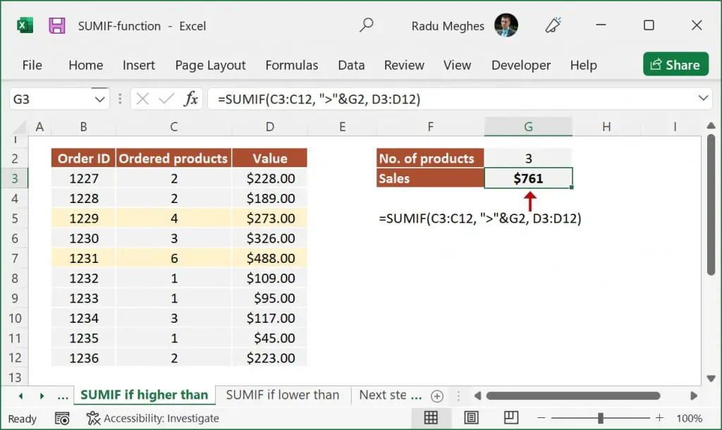
Let’s assume we want to sum up the value of all the sales from customers who ordered more than 3 products. The formula can be written as:
=SUMIF(C3:C12, ">3", D3:D12)or
=SUMIF(C3:C12, ">"&G2, D3:D12)Note: If you are using a cell reference (like G2), you need to concatenate the logical operator with the cell using the ampersand symbol (&).
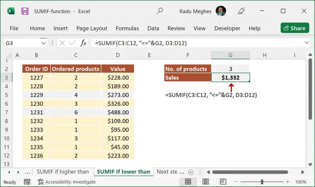
Alternatively, if you want to calculate the sum of all sales from customers who ordered 3 products or less, you can change the SUMIF condition while using the same range argument:
=SUMIF(C3:C12, "<=3", D3:D12)or
=SUMIF(C3:C12, "<="&G2, D3:D12)