How to use IPMT function in Excel [step by step guide]

April 2, 2022June 1, 2022

The tutorial shows how to use IPMT function in Excel to calculate the interest portion for a given period of a loan, mortgage, or investment. The function uses constant payments and a constant interest rate.

This applies to the following Microsoft Excel versions: Excel for Microsoft 365, Excel 2021, 2019, 2016, 2013, 2010, 2007, and 2003.

I recommend downloading the IPTM formula Excel spreadsheet I’ve used to create this tutorial. It makes it easy for you to follow along.

How to use the IPMT function

IPMT is a financial function that returns the interest payment for a loan. IPMT is the abbreviation for interest payment.

The IPMT function uses the following syntax:

=IPMT(rate, per, nper, pv, [fv], [type])

where

• rate (required) – the constant interest rate per period (i.e., the rate corresponding to your payment frequency). For example, if you have a loan with a 6% annual interest rate and yearly payments, then you would use 6% or 0.06; for monthly payment periods, you would need to convert the interest to match the monthly frequency and use 0.5% (6%/12);
• per (required) – the period for which you want to calculate the interest; it must be an integer in the range of 1 to nper;
• nper (required) – the number of payment periods during the lifetime of the loan;
• pv (required) – the present value of the loan; this is the loan principal or the loan amount, i.e., the amount borrowed from the bank.
• fv (optional) – the future value of the balance after the last payment is made;
• type (optional) – specifies when the interest amount is due: 0 for the end of the period and 1 for the beginning of the period.

Note: If omitted, the optional parameters fv and type arguments will use the default value of zero.

How to use the IPMT function in Excel – formula examples

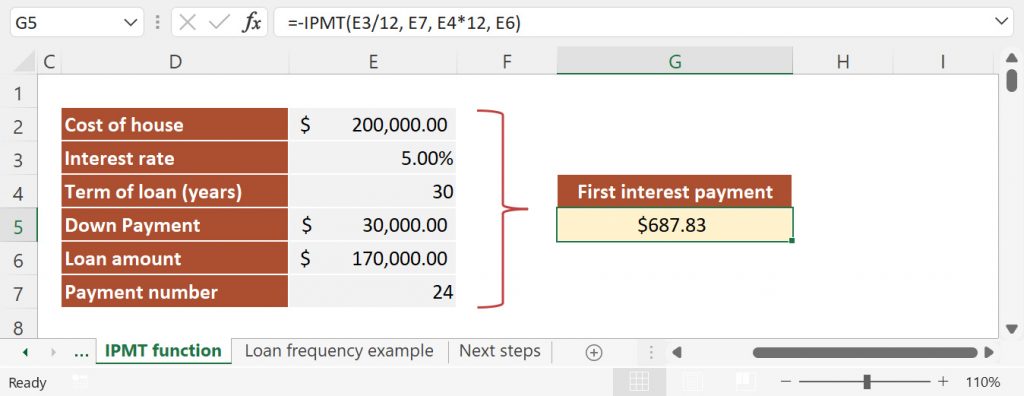
Let’s assume that we have a mortgage loan with a period of 30 years and a constant annual interest rate of 5%. The borrowed amount is $170,000, and payments are due at the end of each month. After the last payment is made, the residual value is $0 (i.e., we want to repay the entire loan).

How to write an IPMT formula in Excel

As I mentioned before, the IPTM function returns the interest portion for a specified period. Let’s say that we want to retrieve the interest due at the end of the second year. This means that our per argument should be 24. You can write the IPMT formula in 7 steps:

1. Use the mouse or keyboard to navigate to the cell where you want to insert the IPMT formula. In my file, this is cell G5.
2. Type =-IPMT(
3. Select the rate argument. Since we use monthly payments, we need to divide the annual rate by 12. In my formula, this corresponds to E3/12.
4. Insert the period for which you want to return the interest paid. In my example, this is 24 (cell E7)
5. Enter the number of periods or the nper argument. In our case, this is E4*12 which is equal to 360 months.
6. Select the present value of the loan or the pv argument. I’ve used cell E6.
7. Type ) to close the function and press ENTER.

When you use the IPMT function to calculate the interest portion of an annuity, you should remember that the returned values are negative because they represent outgoing payments. If you need to show positive numbers, you can simply add the minus sign at the beginning of your formula, which will revert the sign of negative numbers (like I did in the previous example).

Calculate weekly, monthly, quarterly, and semi-annual interest payments

Whenever you use financial functions, it’s essential to make sure that you are setting the correct payment frequency and converting the rate and nper arguments accordingly. I have included a reference table that shows how to convert from annual interest rate and annual payments to weekly, monthly, quarterly, and semi-annual payments:

payment frequency	rate	nper
weekly	annual interest rate / 52	years * 52
monthly	annual interest rate / 12	years * 12
quarterly	annual interest rate / 4	years * 4
semi-annually	annual interest rate / 2	years * 2

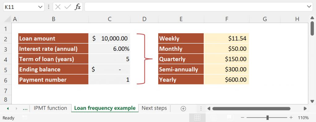
I have prepared an example to demonstrate how the IPMT formula can be adjusted to match different payment frequencies. Let’s calculate the amount of the first interest payment for a $10,000 loan with a 6.00% annual interest rate and duration of 5 years.

Weekly payments:

=-IPMT(6%/52, 1, 5*52, 10000)

Monthly payments:

=-IPMT(6%/12, 1, 5*12, 10000)

Quarterly payments:

=-IPMT(6%/4, 1, 5*4, 10000)

Semi-annual payments:

=-IPMT(6%/2, 1, 5*2, 10000)

Annual payments:

=-IPMT(6%, 1, 5, 10000)

Note: The balance after the last payment (i.e., the fv argument) is assumed to be $0. Interest payments are due at the end of each period, so the type argument is omitted.

Things to remember about the IPMT function

If you want your IPMT formula to work properly you need to consider the following:

• The returned interest payments are negative numbers as Excel follows the cash flow sign convention; you can add the minus sign in front of your formula to convert the result to a positive number;
• The value returned by the IPMT function corresponds to a given period. This is controlled by the per argument.
• The IPMT function can compute the interest of a loan for different frequencies (yearly, quarterly, monthly, weekly); make sure to adjust the total number of periods and convert the annual rate to match your payment frequency.

Excel IPMT function not working properly

If your IPMT formula returns an error or is not working properly, there are several things to check:

• If the result of your IPMT formula looks significantly higher or lower than expected, check to see if your rate and nper arguments are consistent. Using an annual interest rate with monthly payments will return a higher monthly interest payment.
• If your IPMT function returns the #VALUE! error, it means that one of the arguments is non-numeric. Make sure you don’t have numbers stored as text and adjust where necessary.
• If your IPMT function returns the #NUM! error check if the per argument is outside the range of 1 to nper.

What to do next?

The formulas from this Excel tutorial return the interest payment (no principal included). If you want to calculate the total loan payment, you can use the PMT function. Alternatively, you can also calculate the principal payment using the PPMT function and sum the interest and principal payments to get the total loan payment.

If you are having difficulties using the IPMT function, please leave a comment.