How to use IF function with 3 conditions
I received a lot of questions on how to use the IF function with 3 conditions, so I’ve decided to write an article on this topic.
The IF examples described in this article assume that you have a basic understanding of how the IF function works. All examples from this article work in Excel for Microsoft 365 or Excel 2021, 2019, 2016, 2013, 2010, and 2007.
IF is one of the most used Excel functions. In case you are unfamiliar with the IF function, then I strongly recommend reading my article on the Excel IF function first. It’s a step-by-step guide, and it includes a lot of useful examples. It also shows the basics of writing an Excel IF statement with multiple conditions, but it’s not as detailed as this guide. Make sure you also download the exercise file.
As a data analyst, you need to be able to evaluate multiple conditions at the same time and perform an action or display certain values when the logical tests are TRUE. This means that you will need to learn how to write more complex formulas, which sooner or later will include multiple IF statements in Excel, nested one inside the other.
Let’s take a look at how to write a simple IF function with 3 logical tests.
How to use the IF function with 3 conditions
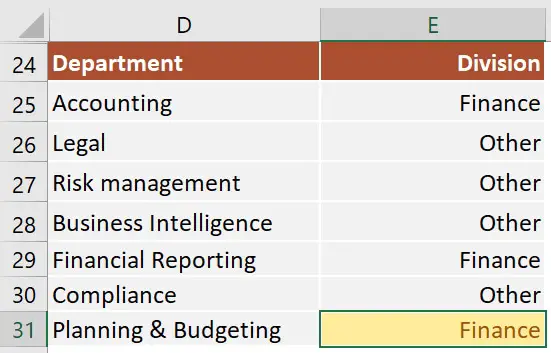
The first example uses an IF statement with three OR conditions. We will use an IF formula which sets the Finance division name if the department is Accounting, Financial Reporting, or Planning & Budgeting.
The IF statement from cell E31 is:=IF(OR(D31="Accounting", D31="Financial Reporting", D31="Planning & Budgeting"), "Finance", "Other")

This IF formula works by checking three OR conditions:
- Is the data from the cell
D31equal toAccounting? In our case, the answer is no, and the formula continues and evaluates the second condition. - Is the text from the cell
D31equal toFinancial Reporting? The answer is still no, and the formula continues and evaluates the third condition. - Is the text from the cell
D31equal toPlanning & Reporting? The answer is yes, our IF function returns TRUE, and displays the word Finance in cell E31.
Next, we focus our attention on an example that uses an IF statement with three AND conditions.
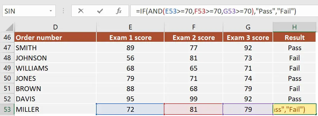
Our table shows exam scores for three exams. If the student received a score of at least 70 for all three exams, then we will return Pass. Otherwise, we will display Fail.
The IF statement from cell H53 is:=IF(AND(E53>=70, F53>=70, G53>=70), "Pass", "Fail")

This IF formula works by checking all three AND conditions:
- Is the score for Exam 1
higher than or equal to 70? In our case, the answer is yes, and the formula continues and evaluates the second condition. - Is the score for Exam 2
higher than or equal to 70? Well, yes it is. Now the formula moves to the third condition. - Is the score for Exam 3 higher than or equal to 70? Yes, it is. Since all three conditions are met, the IF statement is TRUE and returns the word Pass in cell H53.
Excel IF statement with multiple conditions
The final section of this article is focused on how to write an Excel IF statement with multiple conditions, and it includes two examples:
- multiple nested IF statements (also known as nested IFS)
- formula with a mix of AND, OR, and NOT conditions
How many IF statements can you nest in Excel? The answer is 64, but I’ve never seen a formula that uses that many. Also, I’m sure that there are far better alternatives to using such a complicated formula.
Multiple nested IF statements
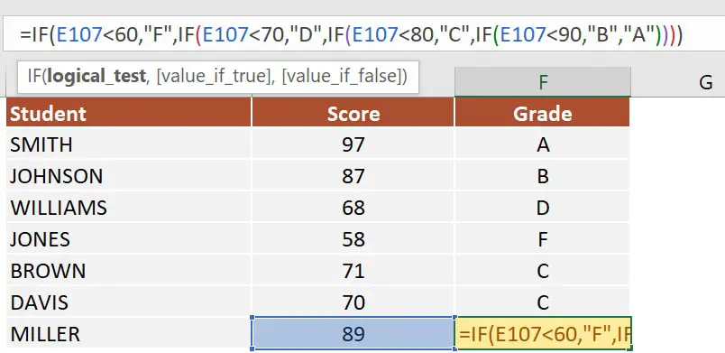
In this example, I have calculated the grades of the students based on their scores using a formula with 4 nested IF functions.
=IF(E107<60, "F", IF(E107<70, "D", IF(E107<80, "C", IF(E107<90, "B" ,"A"))))
Note: In this case, the order of the conditions influences the result of your formula. When your conditions overlap, Excel will return the [value_if_true] argument from the first IF statement that is TRUE and ignores the rest of the values. If you want your formula to work properly, always pay attention to the logical flow and the order of your nested IF functions.
If you have to write an IF statement with 3 outcomes, then you only need to use one nested IF function. The first IF statement will handle the first outcome, while the second one will return the second and the third possible outcomes.

Note: If you have Office 365 installed, then you can also use the new IFS function. You can read more about IFS on Microsoft’s website.
Multiple IF statements in Excel with AND, OR, and NOT conditions
I have saved the best for last. This example is the most advanced from this article, as it involves an IF statement with several other logical functions.
In the exercise file, I have included a list of orders. Each row includes the order date, the order value, the product category, and the free shipping flag. We want to flag orders as eligible if the following cumulative logical conditions are met:
- the order was placed during
2020 - the order includes products from only two categories:
PCorLaptop - the order was
notflagged asFree shipping
The formula I’ve used for cell H80 is shown below:
=IF(AND(D80>=DATE(2020,1,1), D80<=DATE(2020,12,31), OR(F80="PC", F80="Laptop"), NOT(G80="Yes")), "Eligible", "Not eligible")

Here’s how this works:
ANDmakes sure that all the logical conditions need to be met to flag the order as Eligible. If any of them is FALSE, then our entire IF statement will return the [value_if_false] argument.D80>=DATE(2020,1,1)andD80<=DATE(2020,12,31)check if the order was placed between January 1st and December 31st, 2020.ORis used to check whether the product category isPCorLaptop.- Finally,
NOTis used to check if the Free shipping flag is different fromYes.
I’ve also added a video that shows how to nest IF functions in case you are still having difficulties understanding how a nested IF formula works.
And there you have it. I hope that after reading this guide, you have a much better understanding of using IF function with 3 logical tests (or any number actually). While it may seem intimidating at first, I guarantee that if you write an IF formula with multiple criteria daily, your productivity will eventually skyrocket.
This is why, if you have any questions on how to use the IF function with 3 conditions, please leave a comment below and I will do my best to help you out. I reply to every comment or email that I receive.

Hi,
L2 is a cell with either a year or NA, I want to set if L2 is NA or before 2020, it’s Inactive. Then, if Q2 is 0 is active. I have the following formula but it can’t get thru. Appreciated your help.
=IF(L2=NA, “Inactive”, IF(L2<=2020, "Inactive", IF(Q2<0, "Inactive", "Active")))
Hi,
If I understood correctly, if Q2 is 0, then the result should be “active” regardless of the value from L2, which means you should start with that condition. If that is not the case, then please let me know how this should work.
=IF(Q2=0, “Active”, IF(OR(L2=”NA”, L2<=2020), "Inactive", IF(Q2<0, "Inactive", "Active"))) Let me know if that works.
In the previous comment it didnt came out as i wrote. The idea is: if the value in the specified cell is between two values, i want to show 1, if the value in the same specified cell is between two other values, i want to show 2, if the value in the same specified cell is between two other values, i want to show 3 and so on to 5. Thank you in advance.
Hi,
I have created a formula that does what you have asked. Cell C1 is compared with values from cells A1 to A5 and B1 to B5. Just replace the cells in the formula with the ones where you have the values stored, and you should be good to go.
Keep in mind that the formula will return FALSE if the value is not between any of those numbers. I have added the string “Your message” so that you can change it easily. If you prefer, you can also delete this message.
=IF(AND(C1>A1, C1A2, C1A3, C1A4, C1A5, C1
Thank you very much for your reply.
I solved it with this as well:
=IF(K4>=200, “6”, IF(AND(K4>=150, K4=100, K4=50, K4=1, K4<=49), "2", "1"))))))
Hi,
The second part of your formula is weird. Basically, you are checking if K4>=150, K4=100, K4=50, K4=1, K4<=49 simultaneously, and that set of conditions can never be TRUE at the same time. A number can't be equal to 100 and 50 at the same time. This means that the number "2" will never be returned.
In the previous comment it didnt came out as i wrote. The idea is: if the value in the specified cell is between two values, i want to show 1, if the value in the specified cell is between two other values, i want to show 2 and so on to 5.
Thank you in advance.
Hello,
I have some difficulties in nesting these functions, please can you help me?
=IF(AND(K4>Q4, K4R5, K4S5, K4T5, K4U5, K4<V4), "5")
I want to create one function in one cell to do this for me. Am i doing it right or i should look for any other function?
Thank you in advance.
Hi, I would like to know how to write this formula:
Calculate A1 * B1 only if: B1 is > 13, and only if there is at least 3 consecutives values in A1:A6 cells, otherwise put nothing
I really appreciate if you may help me.
Thank you in advance
Hi Chiara,
I think this should work for your scenario:
=IF(B1>13, IF(OR(COUNTA(A1:A3)=3, COUNTA(A2:A4)=3, COUNTA(A3:A5)=3, COUNTA(A4:A6)=3), A1*B1, “”), “”)
Let me know if it worked as intended.
All the best,
Radu
The principal have asked that all students that received an overall grade 80% and above
received the Award ‘Honors’, students with overall grade of 50%-79% received ‘Pass’,
otherwise ‘None’. Insert a column to show this.
Hi Allyan,
I see that you posted the exact same question as Mark. The same formula would apply:
=IF(A1>80%, “Honors”, IF(AND(A1>50%, A1<79%), "Pass", "Fail"))
All the best,
Radu
The principal have asked that all students that received an overall grade 80% and above
received the Award ‘Honors’, students with overall grade of 50%-79% received ‘Pass’,
otherwise ‘None’. Insert a column to show this.
Hi Mark,
I would assume that you need something like this:
=IF(A1>80%, “Honors”, IF(AND(A1>50%, A1<79%), "Pass", "Fail"))
All the best,
Radu
Hi There! Found your site last night when googling the problem I’m trying to fix, but now having trouble with another formula. Excel gave me the lovely popup that there are too many arguments for this function, and I cannot for the life of me find the issue. Could you help me please? In the report, a team member name can be across three columns. If column AH matches either AF or AG or contains “N/A”, I’d like the formula to return the value of “No SS Incentive.” If AH contains a different team member name than AF or AG, then an incentive payment is due. This is the formula I’ve tried using. Could you tell me please what is wrong? Thank you so so much in advance! It stumps me terribly!!
=IF(OR(AH3=”N/A”, “No SS Incentive”), IF(AH3=AF3, “No SS Incentive”), IF(AH3=AG3, “No SS Incentive”),”Sourcing Specialist Incentive Payment Due”))
Hi Nicole,
I think this is the formula you need:
=IF(OR(AH3=”N/A”, AH3=AF3, AH3=AG3), “No SS Incentive”, “Sourcing Specialist Incentive Payment Due”)
There are two issues with your formula. First, you are not using the OR function properly.
Second, your IF Statement had 4 arguments instead of 3. I have broken down your formula into multiple rows so that you can see this more easily.
=IF(OR(AH3=”N/A”, “No SS Incentive”),
IF(AH3=AF3, “No SS Incentive”),
IF(AH3=AG3, “No SS Incentive”),
“Sourcing Specialist Incentive Payment Due”))
Let me know if you need additional help.
All the best,
Radu
Thank you so much, Radu!! You have made my life easier with your help and I cannot thank you enough. Your formula works perfectly! Still learning the ins and outs of formulas, so really appreciate you taking the time to explain the issue and providing the correct formula. Definitely a learning opportunity for me.
Wish you the very best!
Nicole
I am so glad I was able to help. Your feedback has just made my day a lot better 🙂
hi! can you please help me with this:
type a formula that displays “PASSED” if the final grade is greater than or equal “FAILED” if the final grade is less than 70 and “INCOMPLETE” if the final grade is 71 to 74
Hi Abby,
Please use this formula:
=IF(AND(A1>70, A1<74), "INCOMPLETE", IF(A1<=70, "FAILED", " PASSED"))
I would like to run a if function for the following:
if the result in F2 =20 then show “OVER”
Hi Akeem,
Here is the formula:
=IF(F2=20, “OVER”)
All the best,
Radu
please need help on this.
if A1 will have those name then it will automatically type thise letter on C1 with color coding
thanks.
Sean = C
James = Y
John= M
Hi Christine,
The formula you need is:
=IF(A1=”Sean”, “C”, IF(A1=”James”, “Y”, IF(A1=”John”, “M”)))
For color coding, you will have to use Conditional Formatting and add different colors for the cell for each possible letter using a formula like this: =A1=”C”
All the best,
Radu
I am trying to write a formula for the game of baccarat. It has a notorious 3rd card rule to determine whether the “Banker” or the “Player” will take a third card.
The simplest way I can think to do this would basically be…
I have the Player Card in A1, The Banker Card in B1
I am trying to put if A1=0 & B1=0 Then … “Display this text”, if A1=0 & B1 = 0 Then… “Display this different text”
I can get parts of the formula, but every time I try to put it all together, I am getting errors.
Any chance you can help me? I feel like its easier than I’m making it.
I appreciate your help.
Hi Cameron,
What is the difference between A1=0 & B1=0 and A1=0 & B1 = 0? I see the same conditions: A1 must be 0, and B1 must be 0 in both cases.
Radu
Hi. I am trying to write a formula whereby if Tota sales is greater than 2 million, I must insert the text “Acceptable”, if the total sales is greater than 3 million, I insert the text “Amazing”, if the total sales is greater than R3,1 million, I insert the text “Outstanding”.
Hi Sibusiso,
Please find the formula below:
=IF(A1>3100000, “Outstanding”, IF(A1>3000000, “Amazing”, IF(A1>2000000, “Acceptable”, “Message when below 2000000 or delete”)))
You can remove the text “Message when below 2000000 or delete”. That is a placeholder in case you want to display a message if the Total sales are lower than 2 million. Otherwise, the formula would just return FALSE.
Hey how can I use 2 AND statements with an OR statement.
=IF(AND(G2=2016, K2<=2019), IF(AND(G2=2017, K2<=2019), IF(D2<25000, "-", IF(D2<25000, "$200.00", IF(D2<40000, "$225.00", IF(D2=45000, D2*0.0065)))))))
So if G2 less than 78 and is between 2016 – 2019 – OR – if G2 less than 84 and is between 2017-2019.
I keep getting FALSE in the result cell
Hi Gavin,
That is because your first IF statements are not ok. You say =IF(AND(G2=2016, K2<=2019) and add the second IF statement. This tells Excel that if G2=2016 and K2<=2019, it should check if G2=2017 and K2<=2019. Those cannot be true at the same time. From your message I do not understand which cell needs to be between 2016 and 2019 and which below 78 or 84. You message says: "So if G2 less than 78 and is between 2016 - 2019 - OR - if G2 less than 84 and is between 2017-2019." However, in your formula, you check if G2 is equal to 2016 or 2017. Let me know the correct criteria and I'll gladly help you. All the best, Radu
Hello… I am trying to write a formula in excel but unable to do it… Like i have A, B, C, D, E, F so in G col i want the results like.. if col A, C, D is blank i want G col to remain blank and if any Col A, C, D has date G should me the result as Open. And if B, D, E has date it should show result as close… Please help me out… U can show snapshot with the results as well will be very grateful to you ..
Hi Najma,
Try the formula from below and let me know if it works like you want:
=IF(AND(ISBLANK(A1), ISBLANK(C1), ISBLANK(D1)), “”, IF(AND(ISBLANK(B1)=FALSE, ISBLANK(D1)=FALSE, ISBLANK(E1)=FALSE), “Close”, IF(OR(ISBLANK(A1)=FALSE, ISBLANK(C1)=FALSE, ISBLANK(D1)=FALSE), “Open”)))