Count cells not between two numbers
If you are looking to count cells not between two numbers in Excel using COUNTIFS, then you are in for disappointment. That’s because COUNTIFS uses the AND logic when comparing the criteria, resulting in an always FALSE result. And that makes sense since a number can’t be, for example, higher than 100 and lower than 80 simultaneously.
That is why I will show you two alternative formulas: one that joins two COUNTIF statements and a more elegant one using SUMPRODUCT.
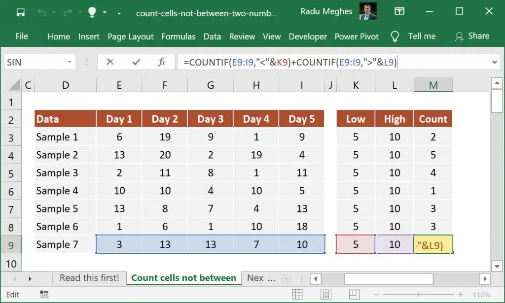
For this, I have created an example of different data samples where we will count observations lower than 5 or higher than 10.
Before we begin, make sure you download the exercise file.
Formula using the COUNTIF function
The syntax is straightforward:=COUNTIF(range, "<"&low)+COUNTIF(range, ">"&high)
where:
range – the range to compare against your criteria;
low – the lower limit of our interval;
high – the lower limit of our interval.

In cell M9, I have inserted the following formula:=COUNTIF(E9:I9, "<"&K9)+COUNTIF(E9:I9, ">"&L9)
The first part checks how many cells have values below our Low value, while the second one checks how many cells contain values above our High value.
Since the operators ">" and "<" are entered as text between double quotes, you must use the ampersand symbol & to concatenate the operator with each number. If you skip this step, Excel will not understand your formula and display an error message.
You can use the same formula to count cells that don’t fall between two dates. All you need to do is replace your numbers with the correct dates, and you are good to go. You can even create dates dynamically using the DATE function.
Formula using the SUMPRODUCT function
SUMPRODUCT is the hidden gem of Excel formulas. It’s so versatile that I can’t stress enough how important it is to master this function. You’ll see in a minute how simple it is to create a more elegant alternative to the COUNTIF combo.

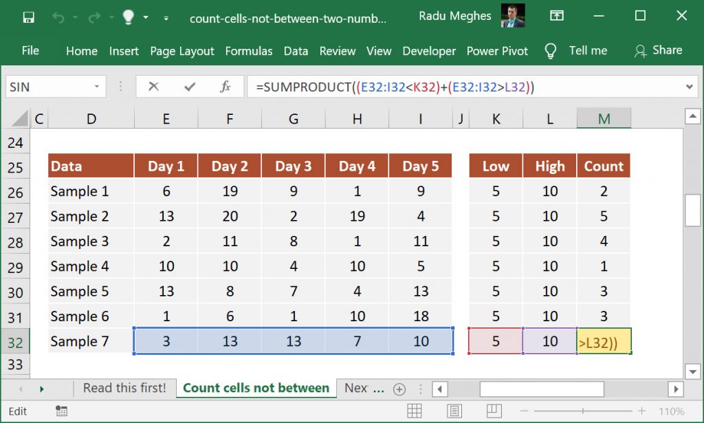
In cell M32, I’ve used the following SUMPRODUCT formula with two logical expressions: =SUMPRODUCT((E32:I32<K32)+(E32:I32>L32))
The first thing to notice is that we don’t need to use concatenation with cell references.
The second thing to remember is that the addition (+) sign used in SUMPRODUCT creates an OR logic.
This formula will evaluate each array and return TRUE or FALSE for each value:
=SUMPRODUCT({TRUE, FALSE, FALSE, FALSE, FALSE} + {FALSE, TRUE, TRUE, FALSE, FALSE})
As you probably know, Excel is programmed to return 1 if the condition is TRUE and 0 if FALSE. This translates our formula into:
=SUMPRODUCT({1, 0, 0, 0, 0} + {0, 1, 1, 0, 0})
Adding the the two arrays results in:
=SUMPRODUCT({1, 1, 1, 0, 0})
The last step is to sum all the items in the array and return the final result of 3.
What to do next?
If you have additional questions about using these formulas or if you still struggle to count cells not between two numbers, please let me know by writing a comment.
