How to wrap text in Excel [step by step]
When you work with a large spreadsheet containing a lot of text that needs to be displayed, long sentences or data strings will either spill over on top of other empty cells on the right or cut off at the cell border if the adjacent cell contains data. This is why it’s important to learn how to wrap text in Excel.

What is wrap text in Excel?
The wrap text feature expands the cells vertically to accommodate all the data on multiple lines. If you’re frequently copying data into an Excel spreadsheet, the wrap text option is helpful because when you paste data into a cell with wrap text formatting enabled, Excel automatically adjusts the width and height of the cell to show all the content.
Where is wrap text in Excel?
There are two ways to activate the wrap text option: the Excel ribbon menu and the Format cells menu. I have covered both in this tutorial, along with the keyboard shortcut that enables text wrapping.
There are several ways to use the Wrap Text option, and the easiest one is from the Excel ribbon. To wrap the text:
1. Select the cells or range of cells you want to format.
2. Go to the Home tab and click the Wrap Text link from the Alignment section.

If you wrap text in cells, the data will automatically adjust to appear on multiple lines within the cell. A wrapped cell expands as you type into it, so it will always display everything you type.
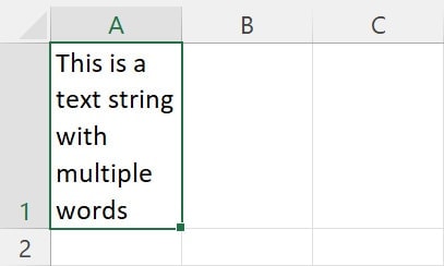
The data wraps to fit the column width automatically, but you can also adjust the width so that the text naturally fits the column width, either by double-clicking the right border of the column header or dragging the column handle.
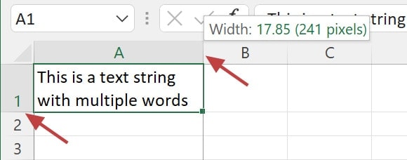
You can also do the same to change the row height by double-clicking the bottom border of the row header.
How to wrap text using a keyboard shortcut
An alternative option is to use a keyboard shortcut to wrap the text inside the cells. To use this method:
1. Highlight the cells or range of cells you want to format.
2. Press , , to apply wrap text formatting. The text wrapping will be automatically applied.
Note: You need to press the keys in consecutive order, not all at once.
Keyboard shortcuts are great because they improve the speed at which you perform actions. I strongly encourage you to learn at least some basic keyboard shortcuts. You’ll soon see that your productivity increases, and you’ll be more inclined to test other shortcuts.
How to wrap text using the Format Cells dialog box
Text wrapping is just another formatting option. You can adjust all the cell formatting from the Format Cells dialog box.
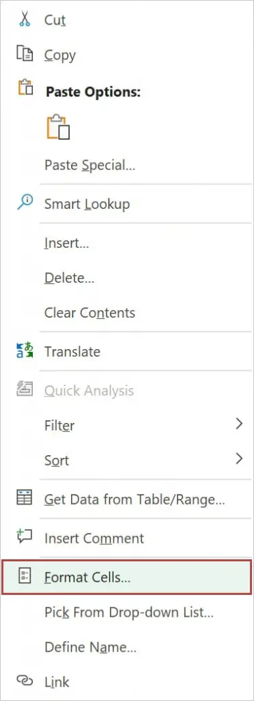
1. Right-click on the cells or range of cells you want to format.
Tip: You can also press + to open the Format Cells dialog box.
2. Choose Format Cells.
3. Check the Wrap text box under the Text control section on the Alignment tab.
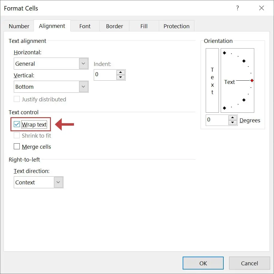
4. Click OK.
Adjusting the cells in the Format Cells dialog box is a better approach if you intend to apply additional formatting rules besides the text wrapping.
Note: A cell that has text wrapping enabled will wrap text automatically until the format is changed or overwritten.
How to wrap text in Excel by adding line breaks
Adding line breaks will automatically adjust the format of your text based on the available width of the cell. This also prevents the column width from getting wider. To do this, simply follow the steps below:
1. Place the cursor in the text at the point where you want to add a line break.

2. Hold the key and press .
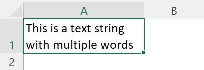
This will add a line break character into your text data and move the remaining text down by one line. You can do this multiple times per cell until you are satisfied with the way your text is displayed.
How to adjust the row height to make wrapped text visible
Sometimes, the text may not be visible because the wrapped text is still too long to fit inside the cell. The limitation of Excel cells will only display the first 1,024 characters. The remaining text is cut off at the border of the cell below. To display the full content, you can increase the row height manually by clicking and dragging the row, but you can also auto-adjust the height by following the steps below:
1. Select the cells or range for which you want to change the row height.
2. Go to the Home tab and click the Format menu in the Cells group.
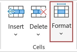
3. Under Cell Size, click AutoFit Row Height from the drop-down menu to modify the row height automatically.
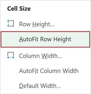
4. If the cells need to have a fixed size, click Row Height under the Cell Size, and type the desired size in the row height box.
The row height will adjust to the exact height needed to show all the text. You can also do the same to adjust the column width by choosing Column Width under the Cell Size and specifying the exact width.
How to remove wrap text formatting
Remove cell formatting
Select the cells or range of cells from which you want to remove the formatting and unwrap the text. Then, navigate to the Home tab and click Wrap Text in the Alignment section to deselect the option.
Alternatively, you can open the Format cells window by pressing + or right-clicking on the cell or range of cells from which you want to remove the formatting. Then, on the Alignment tab, uncheck the Wrap text box under the Text control section and click OK.
If you prefer a keyboard shortcut, you can press , , to remove the wrap text formatting.
Remove line breaks
If you are looking for a quick method to remove the line breaks and the wrap text formatting, follow these steps:
1. Go to the Home tab and click Find & Replace in the Editing group.
Tip: You can also press + to open the Find & Replace window.
2. Place the cursor in the Find what section and press + to add a line break character.
3. Leave the Replace with section empty to remove the line break characters that were added manually.
4. Click Replace All.
What to do next?
Text wrapping greatly improves the way your Excel data is presented, enhancing the readability of your spreadsheet and making data easier to understand. Now that you’ve learned how to wrap text in Excel, there are other helpful Excel tips and tricks that you can apply at work. I recommend further improving your formatting skills by reading the following articles:
